
The recent history of quantum computing has featured a series of claims about reaching "quantum advantage" - the point where quantum computers solve problems that classical computers cannot efficiently handle. However, when examining these claims carefully, we often find that classical algorithms can be improved to match or nearly match quantum performance for specific problems.
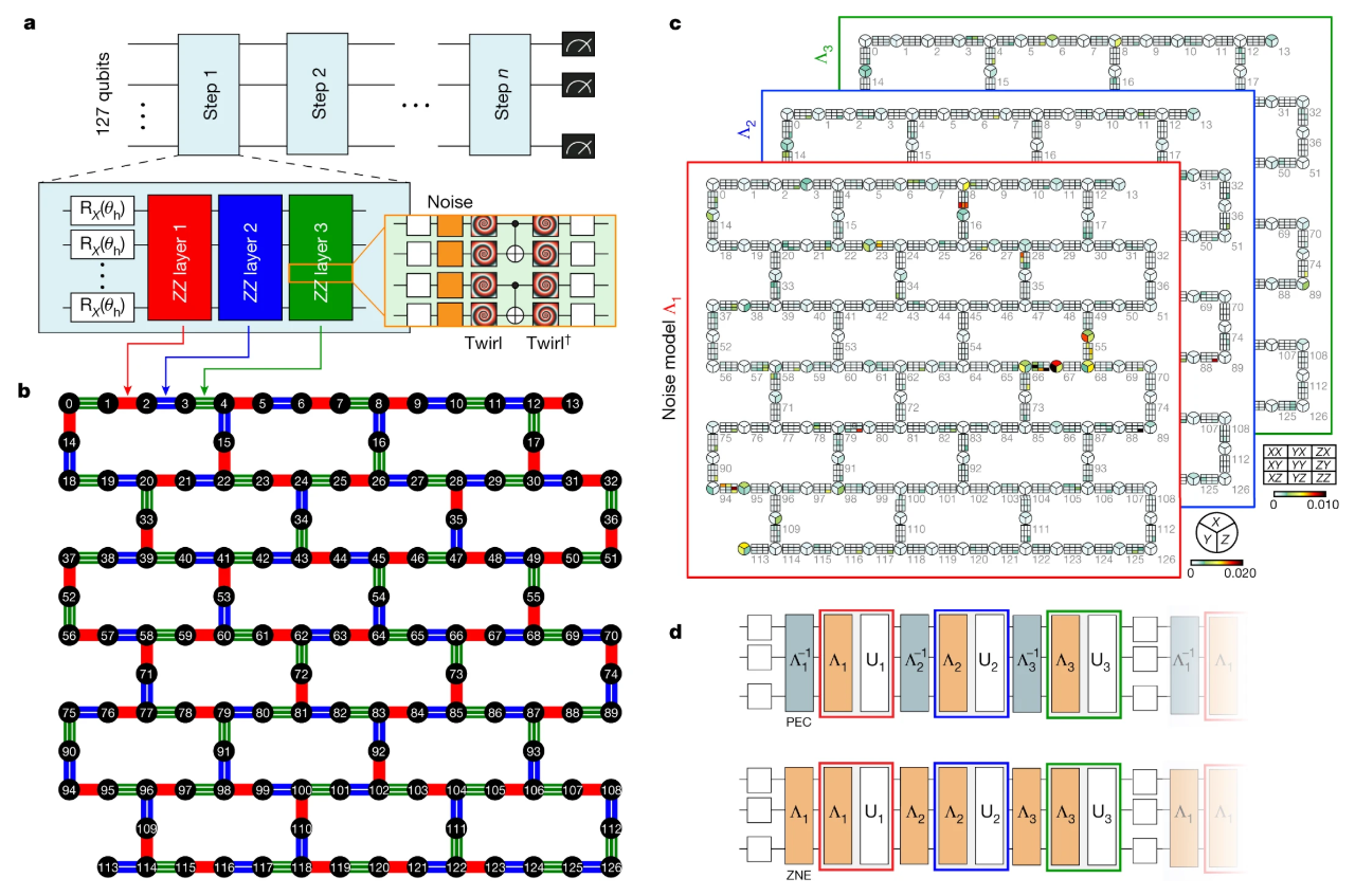
Figure 1: The heavy hexagon lattice of IBM's 127-qubit Eagle processor (b) and Trotterized circuit (d) representing kicked Ising dynamics on the IBM processor that was claimed to demonstrate quantum utility. [Kim et al., Nature 2023]
One notable example is IBM's 2023 paper in Nature by Kim et al., which claimed to demonstrate 'quantum utility' by measuring expectation values on their 127-qubit Eagle processor implementing the kicked Ising model. This claim was subsequently challenged by several research groups, including Caltech, who developed innovative classical simulation techniques that could reproduce the same results on a classical computer substantially faster. These classical methods now serve as essential benchmarking tools for validating quantum utility claims and establishing rigorous baselines for quantum advantage demonstrations.

Before diving into the solution, let's understand the fundamental challenge of classically simulating quantum circuits.
When we evolve a quantum observable through a circuit, we typically express it in terms of Pauli operators. With each gate operation, the number of terms in this Pauli decomposition grows - potentially exponentially with respect to the number of circuit operations.
For example, if we start with a simple observable like σᶻ (Pauli-Z) on a single qubit and apply a Hadamard gate, it transforms into σˣ. But if we continue applying gates across multiple qubits, we can quickly end up with a superposition of thousands or millions of different Pauli strings, each with its own coefficient.
This exponential growth makes brute-force classical simulation infeasible for even moderate-sized quantum circuits, which was the basis for IBM's quantum utility claim.
The key insight is that in most quantum circuits on real hardware affected by noise, complex multi-qubit operations contribute much less to the final result than simpler operations, making it safe to ignore them. This approach offers significant advantages over traditional tensor network and matrix product state methods, which must track all quantum correlations regardless of their importance. Pauli Path Simulators combine multiple smart filtering strategies: removing terms with very small numerical contributions and discarding overly complex multi-qubit operations. Unlike methods that face exponential scaling with entanglement, this selective approach maintains efficiency by focusing computational resources only on the terms that meaningfully affect the final answer, with built-in error monitoring to ensure reliable convergence.
Recent theoretical work by Vazirani, Yao, Holmes, and others has provided rigorous guarantees for such truncation-based approaches. These approaches fall primarily into two categories:
Both approaches share the core principle of tracking only a subset of all possible Pauli paths through the computation, allowing simulation of larger quantum circuits than previously thought possible.
Beyond challenging specific quantum utility claims, Pauli Path Simulators (PPS) serve as powerful benchmarking tools for the quantum computing community. They enable researchers to validate quantum experiments, identify the true boundaries of classical simulation, and design more challenging quantum circuits that may genuinely demonstrate quantum advantage. This benchmarking capability is crucial for the responsible development of quantum computing applications.
The theoretical guarantees for these methods come from several groundbreaking papers. Work by Aharonov, Gao, Landau, Liu, and Vazirani demonstrated that for noisy quantum circuits, classical simulation via Pauli path techniques is efficient.
More remarkably, recent work by Angrisani, Schmidhuber, Rudolph, Cerezo, Holmes, and Huang (2024) established that even for noiseless quantum circuits, Pauli path methods can effectively estimate observables with high accuracy. Their paper "Classically estimating observables of noiseless quantum circuits" shows that for a wide class of quantum circuits - including those with all-to-all connectivity - truncated Pauli path integration achieves small error with high probability.
The key insight is that high-weight Pauli operators' contributions are naturally suppressed in most circuits, making truncation particularly effective.
In the Heisenberg picture used by PPS, we evolve the observable backward through the circuit rather than evolving the quantum state forward. This approach is particularly efficient when the observable is local (like a single Z₆₂ measurement) but the quantum state is highly entangled. For particularly challenging simulations, a mixed Schrödinger/Heisenberg approach can provide optimal efficiency by balancing entanglement between the state and observable.
Our simulator implements our own Pauli Path Simulation (PPS) stack, building on threshold-based Pauli Path simulation concepts originally presented by Garnet Chan's group at Caltech. This implementation is able to simulate the 20-step kicked Ising circuit on 127 qubits in just minutes on a laptop, compared to hours on quantum hardware. At each step of the simulation:
This approach allows us to control memory usage and computational complexity while maintaining excellent accuracy for the final expectation value. For detailed technical implementation and performance analysis, see our paper.
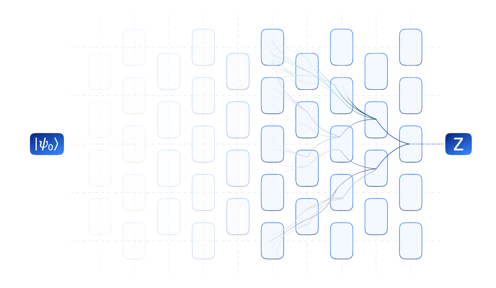
Figure 2: Schematic representation of the Pauli Path simulator. The observable is evolved backwards through the circuit, generically branching to a sum of many operations. These are truncated judiciously and summed up once the circuit has been fully traversed.
We've benchmarked our simulator against results published by leading research groups, including Garnet Chan's implementation. The figure below shows performance comparable to their results, demonstrating that our platform provides state-of-the-art simulation capabilities.
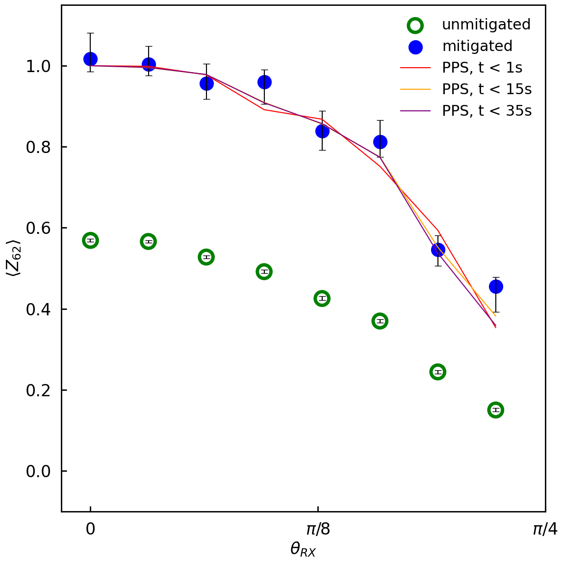
Figure 3: Comparison of expectation values for 〈Z₆₂〉 after 20 circuit steps. BlueQubit’s simulation methods (blue dots) achieve accuracy that matches or exceeds quantum hardware results (green dots). Note that t is the simulation time per choice of θRX, so a larger t means the simulation was done using a smaller threshold.
This plot demonstrates that our coefficient-based truncation method achieves similar accuracy to other published approaches when simulating the circuits from IBM's utility paper. The horizontal axis shows circuit depth, while the vertical axis shows simulation time, illustrating that even deep circuits can be efficiently simulated with our method.
The power of PPS is demonstrated by its ability to achieve absolute accuracy better than 0.01 in the 〈Z₆₂〉 observable for the full 20-step circuit—a level of precision that exceeds the confidence intervals of the quantum hardware results. The most accurate tensor network approaches utilizing the Bethe free entropy formula effectively evaluate expectation values with bond dimensions exceeding 16,000,000, which would be impossible with conventional contraction methods.

Figure 4: Average time scales for simulating IBM's Utility scale experiment for a single θRX. Comparing the 3 methods, Matrix Product State (MPS) required hours, quantum hardware took minutes to hours, and Pauli Path Simulation (PPS) completed in seconds to minutes.
These results have significant implications for claims of quantum advantage. The ability to classically simulate circuits that were previously thought to require quantum computers forces us to reconsider where the true boundary between quantum and classical computation lies.
While there are certainly problems where quantum computers will ultimately demonstrate clear advantages, our work shows that classical techniques are more powerful than often assumed. Claims of quantum advantage require careful verification against the best available classical algorithms.
Our platform makes these advanced simulation techniques accessible with just a click. You can:
This democratizes access to cutting-edge simulation capabilities, allowing researchers, students, and quantum enthusiasts to explore the boundaries of classical simulation.Here is an example code block using the BlueQubit platform to run Pauli Path Simulation:
import numpy as np
from qiskit import QuantumCircuit
import matplotlib.pyplot as plt
import bluequbit

# helper call that returns all the nearest neighbors on the
# IBM 127 qubit system heavy hex lattice
from bluequbit.library.helpers.hardware_connectivites import IBM_127_HEAVY_HEX_MAP

# helper call that returns qiskit Pauli objects given the
# qubits idxs for the X,Y, and Z operators in the Pauli string
from bluequbit.library.helpers.pauli_sum import construct_pauli_from_idx_lists
bq = bluequbit.init (" < API Key >")
num_qubits = 127
num_trotter_steps = 20

# RECREATING THE IBM EXPERIMENT TO ESTIMATE <Z_62>
# Construct a single weight Pauli operator with a Pauli Z at qubit idx 62
idx_lists = [[], [], [62]]
pauli_op = construct_pauli_from_idx_lists(idx_lists, num_qubits)
pauli_sum = [(pauli_op.to_label(), 1.0)]
rzz_angle = -np.pi/2
rx_angle_list = [0, 0.1, 0.2, 0.3, 0.4, 0.5, 0.6, 0.7, 0.8, 1, 1.5707]

# list to store the expectation value <Z_62> for each choice of the rx_angle
expectation_values = []

# set the Pauli path coefficient threshold
options = {
        "pauli_path_truncation_threshold": 8e-4
        }

# construct the circuit for each choice of the rx_angle
for rx_angle in rx_angle_list:
    qc = QuantumCircuit(num_qubits)
    for _ in range(num_trotter_steps):
        for edge in IBM_127_HEAVY_HEX_MAP:
            qc.rzz(rzz_angle, edge[0], edge[1])
        for i in range(num_qubits):
            qc.rx(rx_angle, i)
    # run PPS
    expectation_values.append(
        bq.run(
            qc, device="pauli-path", pauli_sum=pauli_sum, options=options
        ).expectation_value
    )
plt.plot(rx_angle_list, expectation_values)

# RECREATING THE CONVERGENCE CURVE FOR θ_X = 0.3
rzz_angle = -np.pi / 2
rx_angle = 0.3

# list of the coefficient thresholds (delta) in decreasing order
deltas = [1/2** i for i in range(13)]

# list to store the expectation value <Z_62> for each choice of delta
expectation_values = []

# construct circuit for this pair of rzz and rx angles
qc = QuantumCircuit(num_qubits)
for _ in range(num_trotter_steps):
    for edge in IBM_127_HEAVY_HEX_MAP:
        qc.rzz(rzz_angle, edge[0], edge[1])
    for i in range(num_qubits):
        qc.rx(rx_angle, i)
for delta in deltas :
    # set the Pauli path coefficient threshold
    options = {
    " pauli_path_truncation_threshold ": delta ,
    }
    # run PPS
    expectation_values.append(
        bq.run(
            qc, device="pauli-path", pauli_sum=pauli_sum, options=options
        ).expectation_value
    )

plt.plot(-np.log10(deltas), expectation_values)
See our complete implementation and examples on GitHub.
Pauli Path simulation has significant implications for quantum computing investments and research directions:
Our platform democratizes access to these research-grade simulation techniques, allowing organizations of all sizes to benefit from these advanced capabilities without requiring specialized expertise in quantum simulation algorithms.
The development of truncated Pauli path integration represents a significant advance in our ability to classically simulate quantum systems. By intelligently tracking only the most significant contributions to the final result, we can efficiently simulate quantum circuits that were previously thought to be classically intractable.
While quantum computers will ultimately achieve advantages for certain problems, our work pushes the boundary of what's possible with classical computation. Beyond just challenging quantum advantage claims, these simulation methods have valuable applications in algorithm development, hardware validation, and quantum error characterization.
As both quantum hardware and classical algorithms continue to advance, the boundary between quantum and classical advantage will continually evolve, helping focus quantum computing efforts on problems where they provide genuine, practical utility.
Try Bluequbit’s simulation platform today and experience the power of these advanced classical techniques firsthand.


