

The recent history of quantum computing has featured a series of claims about reaching quantum advantage, the point where quantum computers solve problems that classical computers cannot efficiently handle. However, when examining these claims carefully, we sometimes find that advances in classical algorithms can match or approach quantum performance on specific, carefully chosen benchmark circuits, particularly when those circuits have structural properties that classical methods can exploit.
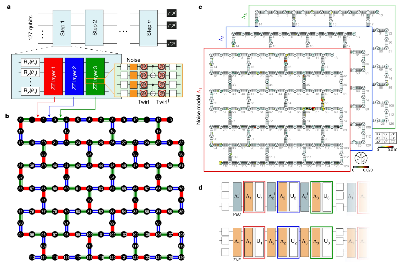
Figure 1: The heavy hexagon lattice of IBM's 127-qubit Eagle processor (b) and Trotterized circuit (d) representing kicked Ising dynamics on the IBM processor that was claimed to demonstrate quantum utility. [Kim et al., Nature 2023]
Pauli Path Simulation gained significant attention following the 2023 study by Kim et al., which examined IBM's utility-scale quantum computing experiment on a 127-qubit processor. IBM had presented the experiment as evidence that quantum hardware was reaching scales difficult for classical computers to reproduce. Using an optimized Pauli Path Simulation approach, however, Begušić & Chan (2025) showed that key aspects of the experiment could be simulated efficiently on classical hardware.
The result did not invalidate IBM's achievement. Instead, it highlighted an important reality in quantum computing: advances in classical simulation algorithms can sometimes narrow the gap between classical and quantum performance. The study demonstrated that the boundary of quantum advantage depends on both hardware progress and the development of increasingly sophisticated simulation techniques.
Before diving into the solution, let's understand the fundamental challenge of classically simulating quantum circuits.
When we evolve a quantum observable through a circuit, we typically express it in terms of Pauli operators. With each gate operation, the number of terms in this Pauli decomposition grows, potentially exponentially with respect to the number of circuit operations.
For example, if we start with a simple observable like σᶻ (Pauli-Z) on a single qubit and apply a Hadamard gate, it transforms into σˣ. But if we continue applying gates across multiple qubits, we can quickly end up with a superposition of thousands or millions of different Pauli strings, each with its own coefficient.
This exponential growth makes brute-force classical simulation infeasible for even moderate-sized quantum circuits, which was the basis for IBM's quantum utility claim.

The key insight is that in most quantum circuits on real hardware affected by noise, complex multi-qubit operations contribute much less to the final result than simpler operations, making it safe to ignore them. This approach offers significant advantages over traditional tensor network and matrix product state methods, which must track all quantum correlations regardless of their importance. Pauli Path Simulators combine multiple smart filtering strategies: removing terms with very small numerical contributions and discarding overly complex multi-qubit operations. Unlike methods that face exponential scaling with entanglement, this selective approach maintains efficiency by focusing computational resources only on the terms that meaningfully affect the final answer, with built-in error monitoring to ensure reliable convergence.
Recent theoretical work by Vazirani, Holmes, and others has provided rigorous guarantees for such truncation-based approaches. These approaches fall primarily into two categories:
Both approaches share the core principle of tracking only a subset of all possible Pauli Paths through the computation, allowing simulation of larger quantum circuits than previously thought possible.
Beyond challenging specific quantum utility claims, Pauli Path Simulators (PPS) serve as powerful benchmarking tools for the quantum computing community. They enable researchers to validate quantum experiments, identify the true boundaries of classical simulation, and design more challenging quantum circuits that may genuinely demonstrate quantum advantage. This benchmarking capability is crucial for the responsible development of quantum computing applications.
Several closely related techniques have been proposed for efficiently simulating quantum circuits by propagating Pauli operators rather than tracking the full quantum state. While they differ in implementation and optimization strategy, they all belong to the same broader family of Pauli-based classical simulation methods.
Pauli Path Simulation (PPS) is not a universal solution for quantum circuit simulation. Its performance depends heavily on the structure of the circuit being analyzed. In general, PPS performs best when three key conditions are met:
PPS typically produces estimates with quantifiable statistical confidence rather than exhaustively calculating every possible quantum state. For many benchmarking, validation, and research tasks, these probabilistic guarantees are sufficient and can dramatically reduce computational costs compared to exact simulation methods.
PPS works particularly well on circuits where quantum information spreads gradually through local interactions rather than becoming instantly distributed across the entire system. In these locally scrambling circuits, Pauli operators remain manageable enough for the simulator to track efficiently.
Shallower circuits generally produce fewer complex Pauli Paths, allowing simulations to remain computationally tractable. As circuit depth increases, the number of possible paths can grow rapidly, increasing simulation time and memory requirements.
One known limitation occurs with deep, highly entangling circuits where quantum information becomes broadly distributed across many qubits. In these cases, the number of relevant Pauli paths can grow exponentially, reducing the efficiency advantage that PPS provides. When this happens, alternative approaches such as tensor network methods, state-vector simulation, or quantum hardware itself may become more practical depending on the problem being studied.
The theoretical guarantees for these methods come from several key papers that established rigorous efficiency guarantees for Pauli-Path truncation — first for noisy circuits, and more recently for noiseless ones. Work by Aharonov, Gao, Landau, Liu, and Vazirani demonstrated that for noisy quantum circuits, classical simulation via Pauli Path techniques is efficient.
More remarkably, recent work by Angrisani, Schmidhuber, Rudolph, Cerezo, Holmes, and Huang (2024) established that even for noiseless quantum circuits, Pauli Path methods can effectively estimate observables with high accuracy. Their paper "Classically estimating observables of noiseless quantum circuits" shows that for a wide class of quantum circuits - including those with all-to-all connectivity - truncated Pauli Path integration achieves small error with high probability.
The key insight is that high-weight Pauli operators' contributions are naturally suppressed in most circuits, making truncation particularly effective.
In the Heisenberg picture used by PPS, we evolve the observable backward through the circuit rather than evolving the quantum state forward. This approach is particularly efficient when the observable is local (like a single Z₆₂ measurement) but the quantum state is highly entangled. For particularly challenging simulations, a mixed Schrödinger/Heisenberg approach can provide optimal efficiency by balancing entanglement between the state and observable.
Traditional quantum simulation often follows the Schrödinger picture, where the quantum state is evolved forward through every gate in the circuit. As the number of qubits grows, tracking the full state becomes increasingly expensive because the state space expands exponentially. The Heisenberg picture takes the opposite approach: instead of evolving the quantum state, it evolves the measurement observable backward through the circuit, a process known as Pauli propagation when the observable is represented using Pauli operators. When only a small number of observables need to be evaluated, this can dramatically reduce the amount of information that must be tracked. In practice, many Pauli Path Simulation implementations use a hybrid approach, combining Schrödinger and Heisenberg evolution to balance computational cost and accuracy depending on the circuit structure and the quantities being measured.
Pauli propagation tracks how a Pauli word changes as it is conjugated by each gate in a quantum circuit. For a gate U and Pauli operator P, Heisenberg-picture evolution is:
P′ = U† P U
For Clifford gates such as CNOT, an input Pauli word maps to another Pauli word, sometimes with a positive or negative sign. This makes the update efficient because the simulator never needs to construct the full quantum state.
Consider a CNOT gate with qubit c as the control and qubit t as the target. Suppose the observable before propagation is:
P = Xc Zt
The CNOT conjugation rules are:
Xc → XcXt
Zt → ZcZt
Applying both transformations gives:
CNOT† (XcZt) CNOT
= (XcXt)(ZcZt)
Operators acting on different qubits commute, so we can regroup them by qubit:
(XcZc)(XtZt)
Using the Pauli multiplication rule:
XZ = −iY
we obtain:
(−iYc)(−iYt) = −YcYt
Therefore:
XcZt → −YcYt
This example shows that propagating a Pauli word involves more than replacing individual operators. The simulator must also track the phase introduced when Pauli operators are multiplied.
These four generator rules are enough to determine how any two-qubit Pauli word transforms through a CNOT gate. More complex Pauli words are propagated by transforming each component, multiplying the results, and keeping track of any resulting sign or phase.
Our simulator implements our own Pauli Path Simulation (PPS) stack, building on threshold-based Pauli Path simulation concepts originally presented by Garnet Chan's group at Caltech. This implementation is able to simulate the 20-step kicked Ising circuit on 127 qubits in just minutes on a laptop, compared to hours on quantum hardware. At each step of the simulation:
This approach allows us to control memory usage and computational complexity while maintaining excellent accuracy for the final expectation value. For detailed technical implementation and performance analysis, see our paper.
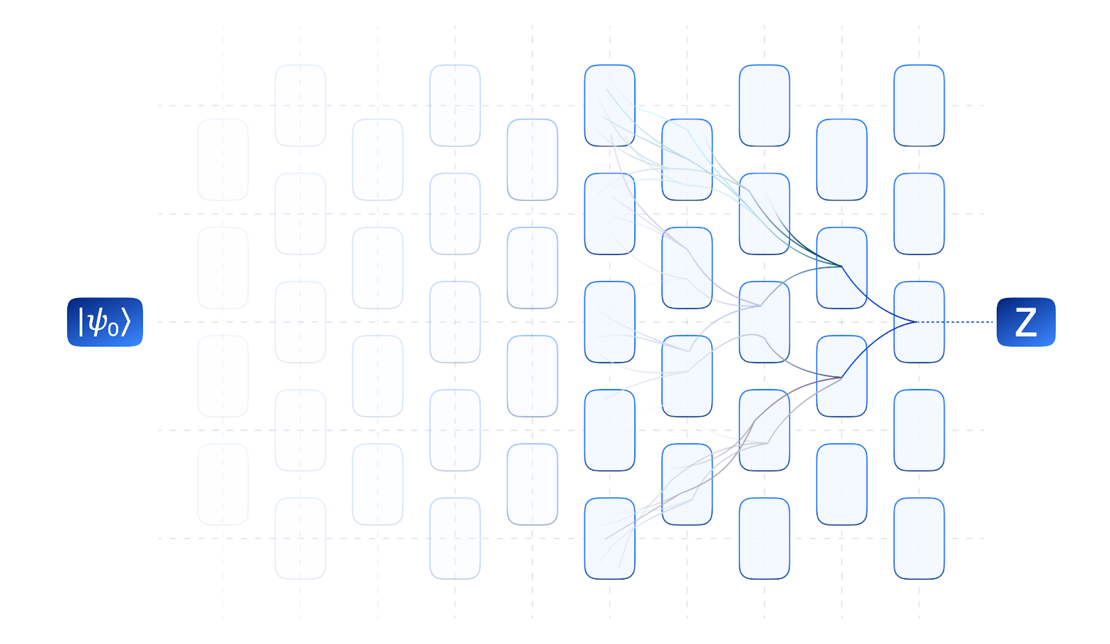
Figure 2: Schematic representation of the Pauli Path Simulator. The observable is evolved backwards through the circuit, generically branching to a sum of many operations. These are truncated judiciously and summed up once the circuit has been fully traversed.
We've benchmarked our simulator against results published by leading research groups, including Garnet Chan's implementation. The figure below shows performance comparable to their results, demonstrating that our platform provides state-of-the-art simulation capabilities.
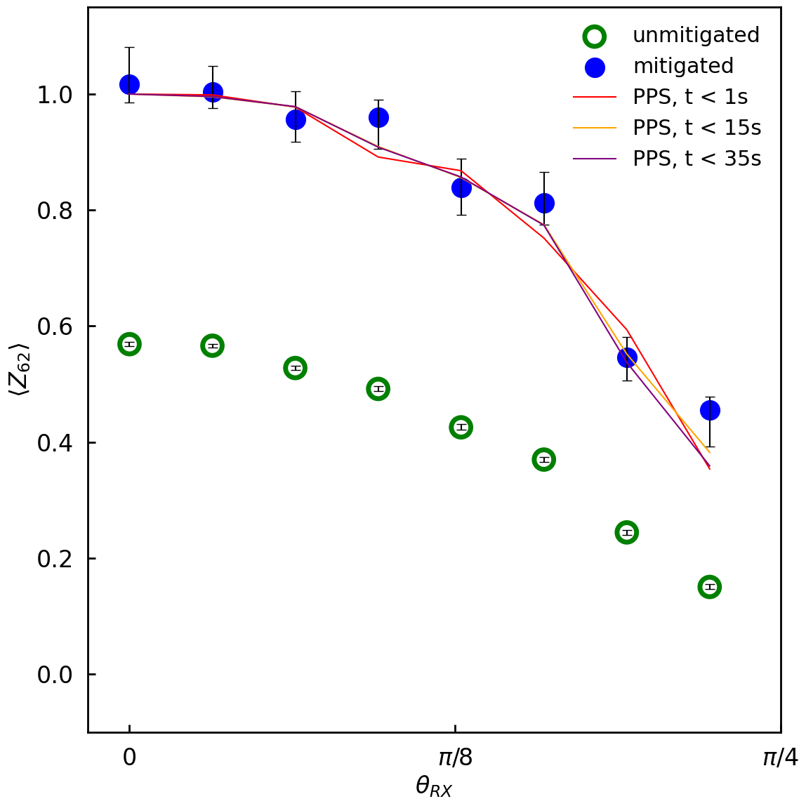
Figure 3: Comparison of expectation values for 〈Z₆₂〉 after 20 circuit steps. BlueQubit’s simulation methods (blue dots) achieve accuracy that matches or exceeds quantum hardware results (green dots). Note that t is the simulation time per choice of θRX, so a larger t means the simulation was done using a smaller threshold.
This plot demonstrates that our coefficient-based truncation method achieves similar accuracy to other published approaches when simulating the circuits from IBM's utility paper.
The truncation threshold controls the trade-off between simulation accuracy and computational efficiency. Lower thresholds retain more Pauli Paths, improving accuracy but increasing runtime and memory usage. Higher thresholds discard more low-contribution paths, accelerating the simulation at the cost of reduced precision. As shown in Figure 3, the convergence curve demonstrates that accuracy improves rapidly as the threshold is lowered before eventually reaching a point of diminishing returns. The value 8 × 10⁻⁴ represents a practical balance, preserving most of the simulation fidelity while avoiding the computational overhead associated with tracking increasingly insignificant contributions.
The power of PPS is demonstrated by its ability to achieve absolute accuracy better than 0.01 in the 〈Z₆₂〉 observable for the full 20-step circuit—a level of precision that exceeds the confidence intervals of the quantum hardware results. The most accurate tensor network approaches utilizing the Bethe free entropy formula effectively evaluate expectation values with bond dimensions exceeding 16,000,000, which would be impossible with conventional contraction methods (Begušić, Gray & Chan).
Figure 4: Average time scales for simulating IBM's Utility scale experiment for a single θRX.
*Representative runtimes based on the IBM Utility-scale 127-qubit benchmark discussed in this article. Actual performance depends on circuit structure, hardware, and simulation settings.
These results have significant implications for claims of quantum advantage. The ability to classically simulate circuits that were previously thought to require quantum computers forces us to reconsider where the true boundary between quantum and classical computation lies.
While there are certainly problems where quantum computers will ultimately demonstrate clear advantages, our work shows that classical techniques are more powerful than often assumed. Claims of quantum advantage require careful verification against the best available classical algorithms.
Our platform makes these advanced simulation techniques accessible with just a click. You can:
This democratizes access to cutting-edge simulation capabilities, allowing researchers, students, and quantum enthusiasts to explore the boundaries of classical simulation. Here is an example code block using the BlueQubit platform to run Pauli Path Simulation:
import numpy as np
from qiskit import QuantumCircuit
import matplotlib.pyplot as plt
import bluequbit

# helper call that returns all the nearest neighbors on the
# IBM 127 qubit system heavy hex lattice
from bluequbit.library.helpers.hardware_connectivites import IBM_127_HEAVY_HEX_MAP

# helper call that returns qiskit Pauli objects given the
# qubits idxs for the X,Y, and Z operators in the Pauli string
from bluequbit.library.helpers.pauli_sum import construct_pauli_from_idx_lists
bq = bluequbit.init (" < API Key >")
num_qubits = 127
num_trotter_steps = 20

# RECREATING THE IBM EXPERIMENT TO ESTIMATE <Z_62>
# Construct a single weight Pauli operator with a Pauli Z at qubit idx 62
idx_lists = [[], [], [62]]
pauli_op = construct_pauli_from_idx_lists(idx_lists, num_qubits)
pauli_sum = [(pauli_op.to_label(), 1.0)]
rzz_angle = -np.pi/2
rx_angle_list = [0, 0.1, 0.2, 0.3, 0.4, 0.5, 0.6, 0.7, 0.8, 1, 1.5707]

# list to store the expectation value <Z_62> for each choice of the rx_angle
expectation_values = []

# set the Pauli path coefficient threshold
options = {
        "pauli_path_truncation_threshold": 8e-4
        }

# construct the circuit for each choice of the rx_angle
for rx_angle in rx_angle_list:
    qc = QuantumCircuit(num_qubits)
    for _ in range(num_trotter_steps):
        for edge in IBM_127_HEAVY_HEX_MAP:
            qc.rzz(rzz_angle, edge[0], edge[1])
        for i in range(num_qubits):
            qc.rx(rx_angle, i)
    # run PPS
    expectation_values.append(
        bq.run(
            qc, device="pauli-path", pauli_sum=pauli_sum, options=options
        ).expectation_value
    )
plt.plot(rx_angle_list, expectation_values)

# RECREATING THE CONVERGENCE CURVE FOR θ_X = 0.3
rzz_angle = -np.pi / 2
rx_angle = 0.3

# list of the coefficient thresholds (delta) in decreasing order
deltas = [1/2** i for i in range(13)]

# list to store the expectation value <Z_62> for each choice of delta
expectation_values = []

# construct circuit for this pair of rzz and rx angles
qc = QuantumCircuit(num_qubits)
for _ in range(num_trotter_steps):
    for edge in IBM_127_HEAVY_HEX_MAP:
        qc.rzz(rzz_angle, edge[0], edge[1])
    for i in range(num_qubits):
        qc.rx(rx_angle, i)
for delta in deltas :
    # set the Pauli path coefficient threshold
    options = {
    " pauli_path_truncation_threshold ": delta ,
    }
    # run PPS
    expectation_values.append(
        bq.run(
            qc, device="pauli-path", pauli_sum=pauli_sum, options=options
        ).expectation_value
    )

plt.plot(-np.log10(deltas), expectation_values)
See our complete implementation and examples on GitHub.
Pauli Path Simulation has significant implications for quantum computing investments and research directions:
Our platform democratizes access to these research-grade simulation techniques, allowing organizations of all sizes to benefit from these advanced capabilities without requiring specialized expertise in quantum simulation algorithms.
Like any classical quantum simulation technique, Pauli Path Simulation (PPS) involves trade-offs between accuracy and computational cost. While it can efficiently simulate many large, low-noise quantum circuits, its performance depends on both the circuit being simulated and the chosen approximation settings.
Pauli Path Simulation controls computational complexity by discarding Pauli terms whose contribution falls below a chosen truncation threshold. As a quantum circuit becomes deeper, more Pauli terms are generated during propagation. Removing small terms keeps the simulation tractable, but it also introduces approximation error. In general, deeper circuits require either a lower truncation threshold to maintain accuracy or acceptance of larger approximation errors.
The theoretical guarantees behind Pauli Path Simulation apply on average across a family of parameterized quantum circuits rather than to every individual circuit instance. While most circuits within the family can be simulated with high accuracy, particular parameter choices may generate more complex Pauli dynamics that are harder to approximate. As a result, the accuracy of any single simulation depends on the specific circuit, its parameters, and the selected truncation settings.
The truncation threshold directly determines how many Pauli terms the simulator retains. A lower threshold preserves more terms, improving simulation accuracy but increasing memory usage and runtime. A higher threshold removes more terms, reducing computational cost at the expense of greater approximation error. In practice, users choose a threshold that balances accuracy and performance for the problem they are solving.
Pauli Path Simulation performs particularly well on low-noise circuits with limited non-Clifford complexity, where the number of significant Pauli terms remains manageable. As circuit complexity grows, the computational advantages gradually diminish because more Pauli operators must be propagated and retained throughout the simulation.
The development of truncated Pauli Path integration is a major leap in our ability to classically simulate quantum systems. By intelligently tracking only the most significant contributions to the final result, we can efficiently simulate quantum circuits that were previously thought to be classically intractable.
While quantum computers will ultimately achieve advantages for certain problems, our work pushes the boundary of what's possible with classical computation. Beyond just challenging quantum advantage claims, these simulation methods have valuable applications in algorithm development, hardware validation, and quantum error characterization.
As both quantum hardware and classical algorithms continue to advance, the boundary between quantum and classical advantage will continually evolve, helping focus quantum computing efforts on problems where they provide genuine, practical utility.
Try Bluequbit’s simulation platform today and experience the power of these advanced classical techniques firsthand.
Pauli Path Simulation is a classical simulation technique that models quantum circuits by representing quantum operations as combinations of Pauli operators. Instead of tracking the full quantum state vector, it follows paths through a space of Pauli transformations, allowing certain quantum circuits to be simulated more efficiently on classical hardware. This approach can significantly reduce computational requirements for specific classes of problems while maintaining accurate results.
Both approaches aim to make quantum circuit simulation more efficient, but they use different mathematical frameworks. Tensor network simulators compress quantum states by exploiting limited entanglement, making them effective for circuits with favorable connectivity patterns. Pauli Path Simulators, on the other hand, analyze how Pauli operators propagate through a circuit and can be particularly effective for circuits with structures that align well with Pauli-based representations. The best method depends on the circuit architecture, entanglement characteristics, and simulation goals.
No. Pauli Path Simulation is a powerful classical tool for studying and validating quantum algorithms, but it still runs on conventional computers and remains subject to classical computational limits. As quantum circuits grow in size and complexity, simulation costs eventually become prohibitive. Quantum hardware is still required to achieve large-scale quantum advantage and solve problems that exceed the capabilities of classical simulation techniques.
Pauli Path Simulators are particularly well-suited for circuits whose operations can be efficiently represented using Pauli-based decompositions. They are often used for benchmarking, algorithm development, error-analysis studies, and validating quantum computations before running them on real quantum hardware. Performance varies depending on circuit depth, gate composition, qubit count, and entanglement structure, so some circuits remain significantly easier to simulate than others.
Pauli Path Simulators help researchers test quantum algorithms, verify results, and explore circuit behavior without requiring access to a physical quantum computer. They provide a practical bridge between theoretical quantum computing and real hardware, enabling faster experimentation, debugging, and performance analysis while quantum processors continue to mature.


